Intended audience: end-users data science developers
AO Easy Answers: 4.4
October 2025
Overview
The Quick Insights library contains 60+ variations of Machine Learning Models, divided into the following 8 groups.
|
Statistical Hypothesis Testing |
Generalized Correlations |
Generalized Regressions |
Causal Inference Analysis |
|---|---|---|---|
|

|
|
|
|
Time-to-Event Analysis |
Geospatial Correlation Analysis |
Univariate Time Series Modeling |
Multivariate Time Series Modeling |
|
|
|
|
Within each group, several variations exist. For example, Causal Analysis supports binary, categorical, and continuous treatments and binary and continuous outcomes.
Details for Each Quick Insight Group
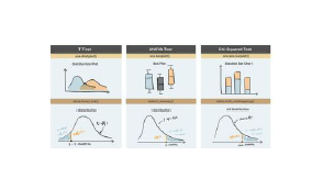
Statistical Hypothesis Testing - 13 Variations
-
Normal Likelihood should be used when:
-
The data is roughly normally distributed and has light tails (i.e., not too many extreme values).
-
You have a large sample size (usually greater than 30).
-
-
Poisson Likelihood should be used when:
-
The data represents count outcomes (e.g., number of incidents, number of occurrences) that are non-negative integers
-
The mean and variance of the data are approximately equal
-
-
Student-T Likelihood should be used when:
-
The data is roughly normally distributed but has heavier tails (i.e., more extreme values or outliers).
-
You have a small sample size (less than 30), where the normal distribution might not be a good approximation.
-
|
Model Name |
Description |
Data Type Requirement |
Example |
|---|---|---|---|
|
One Sample T Test - Normal Likelihood |
Tests if a sample mean differs from a known value. |
Continuous numeric data. |
Testing if the average salary differs from $50,000. |
|
Two Sample T Test - Normal Likelihood |
Tests if two sample means are significantly different. |
Continuous numeric data. |
Comparing average test scores between two schools. |
|
Multi Sample T Test - Normal Likelihood |
Tests if means across multiple groups are significantly different. |
Continuous numeric data. |
Comparing average heights across three different age groups. |
|
One Sample T Test - Poisson Likelihood |
Tests if a sample mean count differs from a known value. |
Discrete count data. |
Testing if the average number of calls per day differs from 10. |
|
Two Sample T Test - Poisson Likelihood |
Tests if two sample mean counts are significantly different. |
Discrete count data. |
Comparing the number of accidents in two regions. |
|
Multi Sample T Test - Poisson Likelihood |
Tests if mean counts differ across multiple groups. |
Discrete count data. |
Comparing accident rates across different districts. |
|
One Sample T Test - Student-T Likelihood |
Tests if a sample mean differs from a known value with heavy-tailed data. |
Continuous numeric data. |
Testing if the mean income differs from $40,000 in a small sample. |
|
Two Sample T Test - Student-T Likelihood |
Tests if two sample means are significantly different with heavy-tailed data. |
Continuous numeric data. |
Comparing income between two small groups. |
|
Multi Sample T Test - Student-T Likelihood |
Tests if means across multiple groups differ with heavy-tailed data. |
Continuous numeric data. |
Comparing income across several cities with heavy variability. |
|
One Sample Binomial Test |
Tests if a sample proportion matches a known proportion. |
Binary categorical data. |
Testing if 60% of the population prefers coffee. |
|
Two Sample Binomial Test |
Tests if two sample proportions differ. |
Binary categorical data. |
Comparing the proportion of smokers in two cities. |
|
Multi Sample Binomial Test |
Tests if proportions across multiple groups differ. |
Binary categorical data. |
Comparing the proportion of defective products across different factories. |
|
Multi Sample Chi2 - Multinomial Test |
Tests if proportions across multiple categories differ. |
Categorical data with more than two categories. |
Testing if the distribution of favorite colors differs across groups. |
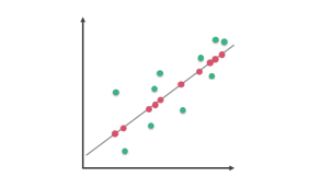
Generalized Correlations - 11 Variations
|
Model Name |
Description |
Data Type Requirement |
Example |
|---|---|---|---|
|
Bayesian Correlation Test (Binary – Binary) |
Measures the degree of association between two binary variables (special case of Pearson’s correlation). |
Both variables must be binary (0/1). |
Relationship between gender (male/female) and whether someone owns a car (yes/no). |
|
Bayesian Correlation Test (Binary – Nominal) |
Quantifies the strength of association between a binary and a nominal variable using chi-square statistics. |
One binary and one nominal variable. |
Association between smoking status (smoker/non-smoker) and favorite beverage type (coffee/tea/soda). |
|
Bayesian Correlation Test (Binary – Continuous) |
Measures the correlation between a binary variable and a continuous variable. Equivalent to Pearson’s correlation when one variable is dichotomous. |
One binary and one continuous numeric variable. |
Correlation between gender (male/female) and salary. |
|
Bayesian Correlation Test (Binary – Ordinal) |
Measures the association between a binary and an ordinal variable by comparing rank distributions across the binary groups. |
One binary variable and one ordinal variable. |
Relationship between treatment type (control/treated) and pain severity (mild/moderate/severe). |
|
Bayesian Correlation Test (Nominal – Nominal) |
Measures the strength of association between two nominal variables using chi-square statistics. |
Both variables must be nominal (categorical without order). |
Association between hair color and favorite cuisine type. |
|
Bayesian Correlation Test (Nominal – Continuous) |
Assesses the strength of association between a nominal and a continuous variable, based on ANOVA concepts. |
One nominal categorical and one continuous numeric variable. |
Relationship between occupation type and annual income. |
|
Bayesian Correlation Test (Ordinal – Continuous) |
Estimates the correlation between an ordinal and a continuous variable, assuming the ordinal variable arises from a latent continuous distribution. |
One ordinal and one continuous variable. |
Association between education level (high school, college, graduate) and test score. |
|
Bayesian Correlation Test (Ordinal – Ordinal) |
Nonparametric measure assessing monotonic association between two ordinal variables. |
Both variables must be ordinal or converted to ranks. |
Correlation between satisfaction level (low, medium, high) and perceived quality (poor, fair, good, excellent). |
|
Bayesian Correlation Test (Continuous – Continuous) |
Computes the correlation between two continuous variables. |
Continuous numeric data. |
Examining the correlation between height and weight. |
|
Bayesian Correlation Test (Nominal – Ordinal) |
Uses Chi2-based association measure between a nominal and an ordinal variable. |
One nominal and one ordinal variable. |
Relationship between region (North, South, East, West) and education level (primary, secondary, tertiary). |
|
Correlation matrix analysis |
Computes the correlation matrix of a set of variables across various data types (binary, nominal, ordinal, and continuous). This can be used to assess variable is highly correlated with a variable of interest (such as a key performance metric). |
Requires tabular data of a set of variables. For practical purposes, the number of variables is restricted to 10. |
Understanding which of my personal and medical features are highly correlated to my heart health. |
Generalized Regressions - 14 Variations
Note: There are two variations in Regressions based on the type of relationship between inputs and output: Linear models (GLM) and Non-linear models (Neural GLM). In GLM, the model parameters have interpretability. Interpretability of parameters in Neural GLM is hard.
-
Poisson Regression
-
The response (output) variable represents counts of events occurring in a fixed time period or a fixed area
-
The mean and variance of counts are approximately equal
-
Example: Number of accidents, Number of visits
-
-
Beta Regression
-
The response variable is continuous and is between 0 and 1
-
Example: Proportions, Rates
-
-
Binomial Regression
-
The response variable represents the number of successful outcomes (or outcomes of interest to us) out of a given number of attempts or trials
-
Example: Number of defective items in a production batch
-
-
Gamma Regression
-
The response variable is continuous, strictly positive, and often right-skewed (heavy right tail)
-
Example: Waiting time
-
-
Negative Binomial Regression
-
The response variable represents count data (similar to Poisson regression)
-
In Poisson regression, the mean and variance are approximately equal
-
Here, the variance is more than the mean (often called overdispersion)
-
Example: Number of insurance claims (with several zeros, some members make more claims than others)
-
-
Bernoulli (Logistic) Regression
-
The response variable is binary
-
We estimate the probability of one outcome as a function of other input predictors
-
Example: Assess whether a customer will purchase a product
-
-
Normal (Linear) Regression
-
The response variable is continuous, and can take any value (positive or negative)
-
Example: Estimating house prices based on size and location
-
|
Model Name |
Description |
Data Type Requirement |
Example |
|---|---|---|---|
|
Poisson Regression (GLM) |
Models count data where events occur at a constant rate. |
Output Data Type: Discrete count data. |
Estimating the number of events (e.g., accidents) at different locations, and modeling the number of customer complaints per day based on weather conditions. |
|
Beta Regression (GLM) |
Models proportions or rates that are bounded between 0 and 1. |
Output Data Type: Continuous data between 0 and 1. |
Estimating the proportion of land covered by vegetation in different regions, and modeling the win percentage in sports based on team statistics. |
|
Binomial Regression (GLM) |
Models success/failure counts out of a fixed number of trials. |
Output Data Type: Count data representing successes out of n trials. |
Modeling the number of students who pass an exam based on study hours. |
|
Gamma Regression (GLM) |
Models continuous data with a skewed distribution, often for time or rate data. Models continuous data that have increasing variance with larger values. |
Output Data Type: Continuous positive data. |
Estimating the time it takes for an event to occur across different locations, and modeling insurance claim amounts based on policyholder age. |
|
Bernoulli (Logistic) Regression (GLM) |
Models binary outcome data with a logistic distribution. |
Output Data Type: Binary categorical data. |
Estimating the likelihood of disease occurrence in different regions. |
|
Normal (Linear) Regression (GLM) |
Models continuous outcome data assuming a normal distribution. |
Output Data Type: Continuous numeric data. |
Estimating the average income across different spatial locations. |
|
Negative Binomial Regression (GLM) |
A regression model for count data with over-dispersion (variance exceeds mean). |
Output Data Type: Discrete count data. |
Modeling the number of customer complaints per week based on weather conditions and staffing levels, when complaints show high variability. |
|
Poisson Regression (Neural GLM) |
Models count data where events occur at a constant rate. |
Output Data Type: Discrete count data. |
Estimating the number of events (e.g., accidents) at different locations, and modeling the number of customer complaints per day based on weather conditions. |
|
Beta Regression (Neural GLM) |
Models proportions or rates that are bounded between 0 and 1. |
Output Data Type: Continuous data between 0 and 1. |
Estimating the proportion of land covered by vegetation in different regions, and modeling the win percentage in sports based on team statistics. |
|
Binomial Regression (Neural GLM) |
Models success/failure counts out of a fixed number of trials. |
Output Data Type: Count data representing successes out of n trials. |
Modeling the number of students who pass an exam based on study hours. |
|
Gamma Regression (Neural GLM) |
Models continuous data with a skewed distribution, often for time or rate data. Models continuous data that have increasing variance with larger values. |
Output Data Type: Continuous positive data. |
Estimating the time it takes for an event to occur across different locations, and modeling insurance claim amounts based on policyholder age. |
|
Bernoulli (Logistic) Regression (Neural GLM) |
Models binary outcome data with a logistic distribution. |
Output Data Type: Binary categorical data. |
Estimating the likelihood of disease occurrence in different regions. |
|
Normal (Linear) Regression (Neural GLM) |
Models continuous outcome data assuming a normal distribution. |
Output Data Type: Continuous numeric data. |
Estimating the average income across different spatial locations. |
|
Negative Binomial Regression (Neural GLM) |
A regression model for count data with over-dispersion (variance exceeds mean). |
Output Data Type: Discrete count data. |
Modeling the number of customer complaints per week based on weather conditions and staffing levels, when complaints show high variability. |
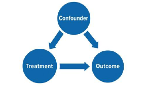
Causal Inference Analysis - 6 Variations: 3 Each for Binary and Continuous Outcomes
Note: In Causal Analysis, we can have binary, categorical, or continuous treatments. Outcome can be binary or continuous. To avoid a lot of combinations, only treatment variations are shown below.
|
Model Name |
Description |
Data Type Requirement |
Example |
|---|---|---|---|
|
Causal Inference with Binary Treatment |
Analyzes the effect of a two-level treatment on an outcome while accounting for factors that influence both treatment assignment and outcome (control variables). |
Treatment: Binary (0/1). Outcome: Continuous or binary. Control Variables: Any combination of continuous, categorical, or binary. |
Estimating the effect of a new drug (treatment vs. control) on blood pressure, considering age, gender, and pre-existing conditions as confounders. |
|
Causal Inference with Categorical Treatment |
Examines the impact of a multi-level treatment on an outcome while controlling for variables that affect both treatment selection and outcome. |
Treatment: Categorical (>2 levels). Outcome: Continuous or binary. Control Variables: Any combination of continuous, categorical, or binary. |
Assessing the effect of different teaching methods (lecture, group work, online) on student test scores, accounting for factors like prior academic performance, socioeconomic status, and school resources. |
|
Causal Inference with Continuous Treatment |
Examines the impact of a continuous treatment on an outcome while controlling for variables that affect both treatment selection and outcome. |
Treatment: Continuous. Outcome: Continuous or binary. Control Variables: Any combination of continuous, categorical, or binary. |
Assessing the effect of exercise time on heart health, accounting for factors like age, education, prior medical conditions, and gender. |
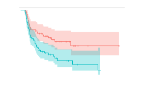
Time-to-Event Analysis - 4 Variations
|
Model Name |
Description |
Data Type Requirement |
Example |
|---|---|---|---|
|
Survival Model with Survival Curve |
Analyzes time until an event occurs, showing the probability of survival over time. |
Time-to-event data, event indicator (0/1). |
Estimating patient survival rates after cancer diagnosis over a 5-year period. |
|
Survival Model + Cohort/Date Effects |
Examines survival patterns across different groups or time periods. |
Time-to-event data, event indicator, cohort/date information. |
Comparing the survival rates of patients diagnosed with a disease in different decades. |
|
Survival Model + Covariates |
Assesses how various factors influence survival time. |
Time-to-event data, event indicator, relevant covariates (numeric/categorical). |
Analyzing how age, gender, and treatment type affect survival time after heart surgery. |
|
Survival Model + Cohort/Date Effects + Covariates |
Combines cohort analysis with factor influence on survival time. |
Time-to-event data, event indicator, cohort/date information, covariates. |
Studying how survival rates for a disease change over decades, considering factors like age, lifestyle, and treatment advances. |
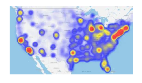
Geospatial Correlation Analysis - 5 Variations
|
Model Name |
Description |
Data Type Requirement |
Example |
|---|---|---|---|
|
Geospatial Gaussian Process Normal |
A model that predicts continuous outcomes at locations by capturing spatial patterns, assuming a normal distribution. |
Response: Continuous data with approximately normal distribution. Inputs: Geographic coordinates (latitude/longitude). Additional Inputs (Optional): Any numeric or categorical, or binary. |
Predicting temperature at different locations in a region, assuming a normal distribution. |
|
Geospatial Gaussian Process Student-T |
A model that predicts continuous outcomes at locations by capturing spatial patterns, robust to outliers and heavy-tailed distributions. |
Response: Continuous data with potential outliers. Inputs: Geographic coordinates (latitude/longitude). Additional Inputs (Optional): Any numeric or categorical, or binary. |
Predicting soil contamination levels across different locations in an industrial area, where some measurements might be extreme. |
|
Geospatial Gaussian Process Poisson |
A model that predicts counts at locations by capturing spatial patterns, suitable for event occurrence data. |
Response: Count data with variance equal to the mean. Inputs: Geographic coordinates (latitude/longitude). Additional Inputs (Optional): Any numeric or categorical, or binary. |
Predicting the number of traffic accidents at different intersections in a city. |
|
Geospatial Gaussian Process Binomial |
A model that predicts binary outcomes at locations by capturing spatial patterns, suitable for presence/absence data. |
Response: Binary data (0/1). Inputs: Geographic coordinates (latitude/longitude). Additional Inputs (Optional): Any numeric or categorical. |
Predicting the presence or absence of a specific plant species across different locations in a forest. |
|
Geospatial Gaussian Process Negative Binomial |
A model that predicts counts at locations by capturing spatial patterns, allowing for overdispersed count data (high variability). |
Response: Count data with variance greater than the mean. Inputs: Geographic coordinates (latitude/longitude). Additional Inputs (Optional): Any numeric or categorical, or binary. |
Predicting the number of disease cases across different locations in a city, where cases tend to cluster spatially and show high variability. |
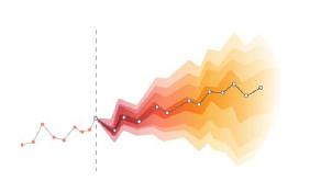
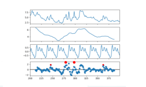
Univariate Time Series Modeling - 6 Variations
|
Model Name |
Description |
Data Type Requirement |
Example |
|---|---|---|---|
|
Univariate Time Series Model with Outlier Detection |
Analyzes a single variable over time, identifying unusual data points, robust to extreme values. |
Single time-ordered variable, timestamps, potential outliers. |
Detecting abnormal spikes in daily stock prices. |
|
Univariate Time Series Model with Change Point |
Detects significant shifts in time series patterns, robust to extreme values. |
Single time-ordered variable, timestamps, potential outliers. |
Identifying when a company's sales pattern fundamentally changed, accounting for occasional extreme sales days. |
|
Univariate Time Series Model with Seasonality/Special Days |
Captures recurring patterns and specific event impacts in time series, robust to extreme values. |
Single time-ordered variable, timestamps, special day indicators. |
Analyzing retail sales considering both yearly seasons and holiday effects, accounting for occasional extreme shopping days. |
|
Univariate Time Series Model with Trend |
Identifies long-term directional movement in time series, robust to extreme values. |
Single time-ordered variable, timestamps, potential outliers. |
Analyzing global temperature changes over decades, accounting for occasional extreme weather events. |
|
Univariate Time Series Model with Exogenous Variables |
Predicts a single variable over time using external factors, robust to outliers, assuming a heavy-tailed distribution (Student-T distribution). |
Time-ordered target variable, relevant external variables. |
Forecasting energy consumption using temperature and economic indicators, accounting for extreme weather events. |
|
Univariate Time Series Model Forecasting |
Projects future values of a single variable based on its past behavior and patterns. |
Time-ordered single variable data, sufficient historical data to capture patterns. |
Predicting future stock prices based on historical price data. |
Multivariate Time Series Modeling - 10 Variations
|
Model Name |
Description |
Data Type Requirement |
Example |
|---|---|---|---|
|
MV Time Series Model with Outlier Detection - Student-T Likelihood |
A model that analyzes multiple related time series, identifies unusual data points, and handles heavy-tailed distributions. |
Multiple related time series, potential outliers, and non-normal distribution. |
Analyzing stock prices of multiple companies in the same industry, detecting market anomalies while accounting for extreme price movements. |
|
MV Time Series Model with Correlations - Student-T Likelihood |
A model that captures relationships between multiple time series while accommodating heavy-tailed distributions. |
Multiple related time series, potential correlations, and non-normal distribution. |
Studying the interdependencies of various economic indicators across different countries, allowing for extreme events. |
|
MV Time Series Model with Change Point - Student-T Likelihood |
A model that detects significant shifts in multiple related time series while handling heavy-tailed distributions. |
Multiple related time series, potential structural changes, and non-normal distribution. |
Identifying policy changes affecting multiple economic indicators simultaneously, accounting for extreme fluctuations. |
|
MV Time Series Model with Seasonality/Special Days - Student-T Likelihood |
A model that accounts for recurring patterns and specific events in multiple time series while handling heavy-tailed distributions. |
Multiple related time series, seasonal patterns, special events, and non-normal distribution. |
Analyzing retail sales across multiple product categories, considering holidays and seasonal trends, while allowing for extreme sales days. |
|
MV Time Series Model with Global and Local Trend - Student-T Likelihood |
A model that captures both overall and series-specific trends in multiple time series while accommodating heavy-tailed distributions. |
Multiple related time series, global and local trends, non-normal distribution, minimum of 3 years of data. |
Studying global and country-specific GDP growth trends, allowing for extreme economic events. |
|
MV Time Series Model with Outlier Detection - Normal Likelihood |
A model that analyzes multiple related time series and identifies unusual data points, assuming normal distribution. |
Multiple related time series, potential outliers, and approximately normal distribution. |
Monitoring sensor readings from multiple machines in a factory, detecting anomalies that may indicate equipment failure. |
|
MV Time Series Model with Correlations - Normal Likelihood |
A model that captures relationships between multiple time series, assuming a normal distribution. |
Multiple related time series, potential correlations, and approximately normal distribution. |
Analyzing the relationships between temperature, humidity, and energy consumption in multiple buildings. |
|
MV Time Series Model with Change Point - Normal Likelihood |
A model that detects significant shifts in multiple related time series, assuming a normal distribution. |
Multiple related time series, potential structural changes, and approximately normal distribution. |
Identifying changes in consumer behavior across multiple product categories following a major marketing campaign. |
|
MV Time Series Model with Seasonality/Special Days - Normal Likelihood |
A model that accounts for recurring patterns and specific events in multiple time series, assuming normal distribution. |
Multiple related time series, seasonal patterns, special events, and approximately normal distribution. |
Forecasting electricity demand for multiple regions, considering seasonal patterns and holidays. |
Contact App Orchid | Disclaimer